反向传播

说到神经网络，大家看到这个图应该不陌生：

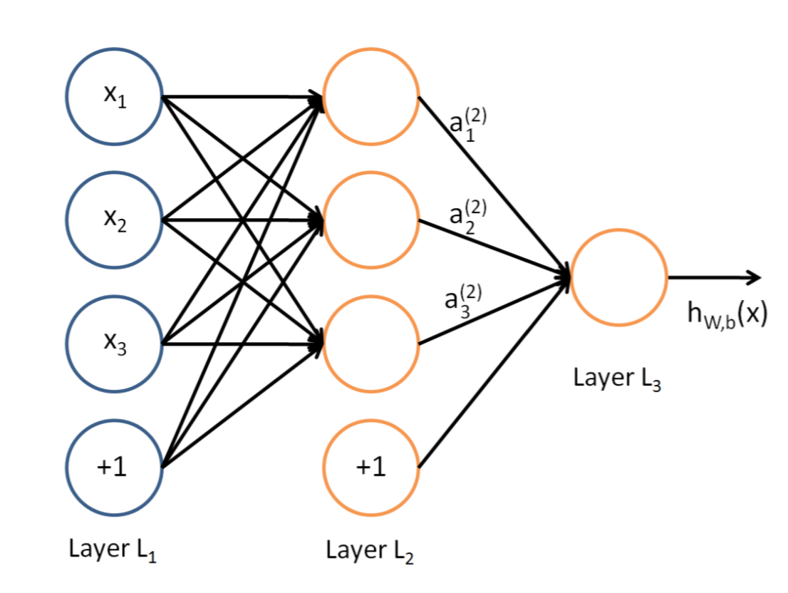
这是典型的三层神经网络的基本构成，Layer L1是输入层，Layer L2是隐含层，Layer L3是隐含层，我们现在手里有一堆数据{x1,x2,x3,…,xn},输出也是一堆数据{y1,y2,y3,…,yn},现在要他们在隐含层做某种变换，让你把数据灌进去后得到你期望的输出。如果你希望你的输出和原始输入一样，那么就是最常见的自编码模型（Auto-Encoder）。可能有人会问，为什么要输入输出都一样呢？有什么用啊？其实应用挺广的，在图像识别，文本分类等等都会用到，我会专门再写一篇Auto-Encoder的文章来说明，包括一些变种之类的。如果你的输出和原始输入不一样，那么就是很常见的人工神经网络了，相当于让原始数据通过一个映射来得到我们想要的输出数据，也就是我们今天要讲的话题。

本文直接举一个例子，带入数值演示反向传播法的过程，公式的推导等到下次写Auto-Encoder的时候再写，其实也很简单，感兴趣的同学可以自己推导下试试：）（注：本文假设你已经懂得基本的神经网络构成，如果完全不懂，可以参考Poll写的笔记：[Mechine Learning & Algorithm] 神经网络基础）

假设，你有这样一个网络层：

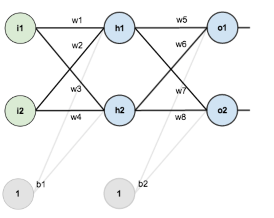
第一层是输入层，包含两个神经元i1，i2，和截距项b1；第二层是隐含层，包含两个神经元h1,h2和截距项b2，第三层是输出o1,o2，每条线上标的wi是层与层之间连接的权重，激活函数我们默认为sigmoid函数。

现在对他们赋上初值，如下图：

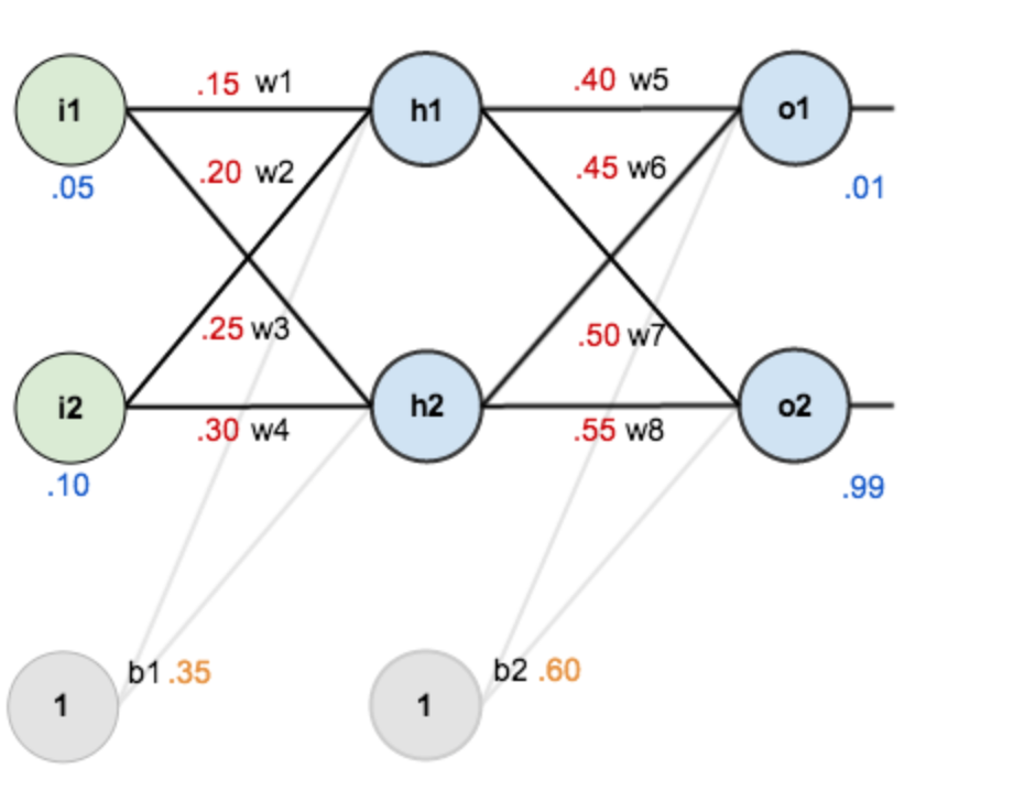
其中，输入数据 i1=0.05，i2=0.10;

　　　输出数据 o1=0.01,o2=0.99;

　　　初始权重 w1=0.15,w2=0.20,w3=0.25,w4=0.30;

　　　　　　　 w5=0.40,w6=0.45,w7=0.50,w8=0.55

目标：给出输入数据i1,i2(0.05和0.10)，使输出尽可能与原始输出o1,o2(0.01和0.99)接近。

Step 1 前向传播

1.输入层—->隐含层：

计算神经元h1的输入加权和： $$ \begin{array}{l} n e t_{h 1}=w_{1} * i_{1}+w_{2} * i_{2}+b_{1} * 1 \
{ net }_{h 1}=0.15 * 0.05+0.2 * 0.1+0.35 * 1=0.3775 \end{array} $$ 神经元h1的输出o1:(此处用到激活函数为sigmoid函数)： $$ { out }_{h 1}=\frac{1}{1+e^{-n e t_{h 1}}}=\frac{1}{1+e^{-0.3775}}=0.593269992 $$ 同理，可计算出神经元h2的输出o2： $$ { out }_{h 2}=0.596884378 $$ 2.隐含层—->输出层：

计算输出层神经元o1和o2的值： $$ \begin{array}{l} { net }{o 1}=w{5} * { out }{h 1}+w{6} * { out }{h 2}+b{2} * 1 \
{ net }{o 1}=0.4 * 0.593269992+0.45 * 0.596884378+0.6 * 1=1.105905967 \
{ out }{o 1}=\frac{1}{1+e^{-n e t_{o 1}}}=\frac{1}{1+e^{-1.105905967}}=0.75136507 \
{ out }_{o 2}=0.772928465 \end{array} $$ 这样前向传播的过程就结束了，我们得到输出值为[0.75136079 , 0.772928465]，与实际值[0.01 , 0.99]相差还很远，现在我们对误差进行反向传播，更新权值，重新计算输出。

Step 2 反向传播

1.计算总误差

总误差：(square error) $$ E_{ {total }}=\sum \frac{1}{2}( { target }- { output })^{2} $$ 但是有两个输出，所以分别计算o1和o2的误差，总误差为两者之和： $$ \begin{array}{l} E_{o 1}=\frac{1}{2}\left( { target }_{o 1}- { out }_{o 1}\right)^{2}=\frac{1}{2}(0.01-0.75136507)^{2}=0.274811083 \
E_{o 2}=0.023560026 \
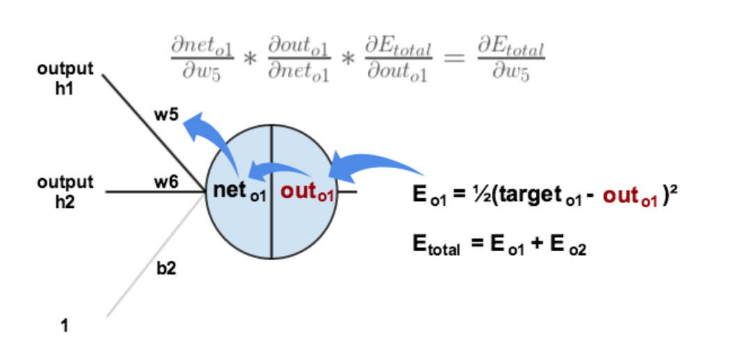
E_{ {total }}=E_{o 1}+E_{o 2}=0.274811083+0.023560026=0.298371109 \end{array} $$ 2.隐含层—->输出层的权值更新：

以权重参数w5为例，如果我们想知道w5对整体误差产生了多少影响，可以用整体误差对w5求偏导求出：（链式法则） $$ \frac{\partial E_{{total }}}{\partial w_{5}}=\frac{\partial E_{\text {total }}}{\partial { out }_{o 1}} * \frac{\partial {out }_{o 1}}{\partial { net }_{o 1}} * \frac{\partial { net }_{o 1}}{\partial w_{5}} $$ 下面的图可以更直观的看清楚误差是怎样反向传播的：

现在我们来分别计算每个式子的值：

计算： $$ \frac{\partial E_{ {total }}}{\partial { out }_{o 1}} $$

$$ \begin{array}{l} E_{ {total }}=\frac{1}{2}\left( { target }_{o 1}-\text { out }_{o 1}\right)^{2}+\frac{1}{2}\left( { target }_{o 2}- { out }_{o 2}\right)^{2} \
\frac{\partial E_{ {total }}}{\partial { out }_{o 1}}=2 * \frac{1}{2}\left( { target }_{o 1}- { out }_{o 1}\right)^{2-1} *-1+0 \
\frac{\partial E_{ {total }}}{\partial { outo }}=-\left( { target }_{o 1}- { out }_{o 1}\right)=-(0.01-0.75136507)=0.74136507 \end{array} $$

计算： $$ \frac{\partial { out }{o 1}}{\partial n e t{o 1}} $$

$$ \begin{array}{l} { out }{o 1}=\frac{1}{1+e^{-n e t{o 1}}} \
\frac{\partial { out }{o 1}}{\partial { net }{o 1}}= { out }{o 1}\left(1- { out }{o 1}\right)=0.75136507(1-0.75136507)=0.186815602 \end{array} $$

（这一步实际上就是对sigmoid函数求导，比较简单，可以自己推导一下）

计算： $$ \frac{\partial { net }{o 1}}{\partial w{5}} $$

$$ \begin{array}{l} n e t_{o 1}=w_{5} * { out }_{h 1}+w_{6} * { out }_{h 2}+b_{2} * 1 \
\frac{\partial { net }_{o 1}}{\partial w_{5}}=1 * { out }_{h 1} * w_{5}^{(1-1)}+0+0= { out }_{h 1}=0.593269992 \end{array} $$

最后三者相乘： $$ \begin{array}{l} \frac{\partial E_{ {total }}}{\partial w_{5}}=\frac{\partial E_{ {total }}}{\partial o u t_{o 1}} * \frac{\partial { out }_{o 1}}{\partial n e t_{o 1}} * \frac{\partial n e t_{o 1}}{\partial w_{5}} \
\frac{\partial E_{ {total }}}{\partial w_{5}}=0.74136507 * 0.186815602 * 0.593269992=0.082167041 \end{array} $$ 这样我们就计算出整体误差E(total)对w5的偏导值。

回过头来再看看上面的公式，我们发现： $$ \frac{\partial E_{t o t a l}}{\partial w_{5}}=-\left(\operatorname{target}_{o 1}- { out }_{o 1}\right) * { out }_{o 1}\left(1- { out }_{o 1}\right) * { out }_{h 1} $$ 为了表达方便，用$$\delta_{o 1}$$来表示输出层的误差： $$ \begin{array}{l} \delta_{o 1}=\frac{\partial E_{ {total }}}{\partial o u t_{o 1}} * \frac{\partial { out }_{o 1}}{\partial n e t_{o 1}}=\frac{\partial E_{ {total }}}{\partial n e t_{o 1}} \
\delta_{o 1}=-\left(\operatorname{target}_{o 1}- { out }_{o 1}\right) * { out }_{o 1}\left(1- { out }_{o 1}\right) \end{array} $$ 因此，整体误差E(total)对w5的偏导公式可以写成： $$ \frac{\partial E_{ {total }}}{\partial w_{5}}=\delta_{o 1} { out }_{h 1} $$ 如果输出层误差计为负的话，也可以写成： $$ \frac{\partial E_{ {total }}}{\partial w_{5}}=-\delta_{o 1} { out }_{h 1} $$ 最后我们来更新w5的值： $$ w_{5}^{+}=w_{5}-\eta * \frac{\partial E_{ {total }}}{\partial_{w_{5}}}=0.4-0.5 * 0.082167041=0.35891648 $$ （其中，$$\eta$$是学习速率，这里我们取0.5）

同理，可更新w6,w7,w8: $$ \begin{array}{l} w_{6}^{+}=0.408666186 \
w_{7}^{+}=0.511301270 \
w_{8}^{+}=0.561370121 \end{array} $$ 3.隐含层—->输入层的权值更新：

　方法其实与上面说的差不多，但是有个地方需要变一下，在上文计算总误差对w5的偏导时，是从out(o1)—->net(o1)—->w5,但是在隐含层之间的权值更新时，是out(h1)—->net(h1)—->w1,而out(h1)会接受E(o1)和E(o2)两个地方传来的误差，所以这个地方两个都要计算。

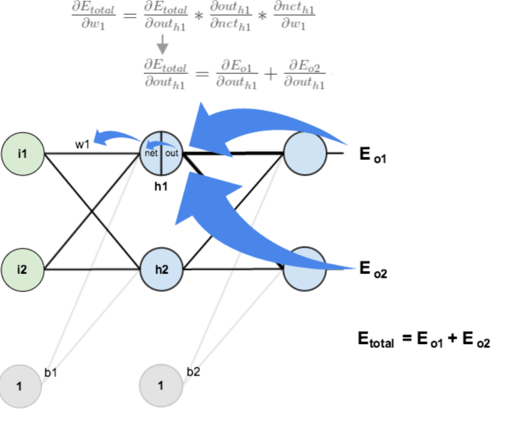
计算： $$ \frac{\partial E_{ {total }}}{\partial { out }_{h 1}} $$

$$ \frac{\partial E_{ {total }}}{\partial o u t_{h 1}}=\frac{\partial E_{o 1}}{\partial o u t_{h 1}}+\frac{\partial E_{o 2}}{\partial o u t_{h 1}} $$

先计算： $$ \frac{\partial E_{o 1}}{\partial o u t_{h 1}} $$

$$ \begin{array}{l} \frac{\partial E_{o 1}}{\partial o u t_{h 1}}=\frac{\partial E_{o 1}}{\partial n e t_{o 1}} * \frac{\partial n e t_{o 1}}{\partial o u t_{h 1}} \
\frac{\partial E_{o 1}}{\partial n e t_{o 1}}=\frac{\partial E_{o 1}}{\partial o u t_{o 1}} * \frac{\partial o u t_{o 1}}{\partial n e t_{o 1}}=0.74136507 * 0.186815602=0.138498562 \
{ net }_{o 1}=w_{5} * o u t_{h 1}+w_{6} * { out }_{h 2}+b_{2} * 1 \
\frac{\partial { net }_{o 1}}{\partial o u t_{h 1}}=w_{5}=0.40 \
\frac{\partial E_{o 1}}{\partial o u t_{h 1}}=\frac{\partial E_{o 1}}{\partial n e t_{o 1}} * \frac{\partial n e t_{o 1}}{\partial o u t_{h 1}}=0.138498562 * 0.40=0.055399425 \end{array} $$

同理，计算出： $$ \frac{\partial E_{o 2}}{\partial o u t_{h 1}}=-0.019049119 $$ 两者相加得到总值： $$ \frac{\partial E_{ {total }}}{\partial o u t_{h 1}}=\frac{\partial E_{o 1}}{\partial o u t_{h 1}}+\frac{\partial E_{o 2}}{\partial o u t_{h 1}}=0.055399425+-0.019049119=0.036350306 $$ 再计算： $$ \frac{\partial o u t_{h 1}}{\partial n e t_{h 1}} $$

$$ \begin{array}{l} { out }{h 1}=\frac{1}{1+e^{-n e t}{h 1}} \
\frac{\partial { out }{h 1}}{\partial n e t{h 1}}= { out }{h 1}\left(1- { out }{h 1}\right)=0.59326999(1-0.59326999)=0.241300709 \end{array} $$

再计算： $$ \frac{\partial n e t_{h 1}}{\partial w_{1}} $$

$$ \begin{array}{l} { net }{h 1}=w{1} * i_{1}+w_{2} * i_{2}+b_{1} * 1 \
\frac{\partial n e t_{h 1}}{\partial w_{1}}=i_{1}=0.05 \end{array} $$

最后，三者相乘： $$ \begin{array}{l} \frac{\partial E_{ {total }}}{\partial w_{1}}=\frac{\partial E_{ {total }}}{\partial { out }_{h 1}} * \frac{\partial { out }_{h 1}}{\partial n e t_{h 1}} * \frac{\partial { net }_{h 1}}{\partial w_{1}} \
\frac{\partial E_{ {total }}}{\partial w_{1}}=0.036350306 * 0.241300709 * 0.05=0.000438568 \end{array} $$ 为了简化公式，用sigma(h1)表示隐含层单元h1的误差： $$ \begin{array}{l} \frac{\partial E_{ {total }}}{\partial w_{1}}=\left(\sum_{o} \frac{\partial E_{ {total }}}{\partial o u t_{o}} * \frac{\partial { out }_{o}}{\partial n e t_{o}} * \frac{\partial { net }_{o}}{\partial o u t_{h 1}}\right) * \frac{\partial o u t_{h 1}}{\partial n e t_{h 1}} * \frac{\partial n e t_{h 1}}{\partial w_{1}} \
\frac{\partial E_{ {total }}}{\partial w_{1}}=\left(\sum_{o} \delta_{o} * w_{h o}\right) * { out }_{h 1}\left(1- { out }_{h 1}\right) * i_{1} \
\frac{\partial E_{ {total }}}{\partial w_{1}}=\delta_{h 1} i_{1} \end{array} $$ 最后，更新w1的权值： $$ w_{1}^{+}=w_{1}-\eta * \frac{\partial E_{\text {total }}}{\partial w_{1}}=0.15-0.5 * 0.000438568=0.149780716 $$ 同理，额可更新w2,w3,w4的权值： $$ \begin{array}{l} w_{2}^{+}=0.19956143 \
w_{3}^{+}=0.24975114 \
w_{4}^{+}=0.29950229 \end{array} $$ 　　这样误差反向传播法就完成了，最后我们再把更新的权值重新计算，不停地迭代，在这个例子中第一次迭代之后，总误差E(total)由0.298371109下降至0.291027924。迭代10000次后，总误差为0.000035085，输出为0.015912196,0.984065734,证明效果还是不错的。

#coding:utf-8
import random
import math

#
#   参数解释：
#   "pd_" ：偏导的前缀
#   "d_" ：导数的前缀
#   "w_ho" ：隐含层到输出层的权重系数索引
#   "w_ih" ：输入层到隐含层的权重系数的索引

class NeuralNetwork:
    LEARNING_RATE = 0.5

    def __init__(self, num_inputs, num_hidden, num_outputs, hidden_layer_weights = None, hidden_layer_bias = None, output_layer_weights = None, output_layer_bias = None):
        self.num_inputs = num_inputs

        self.hidden_layer = NeuronLayer(num_hidden, hidden_layer_bias)
        self.output_layer = NeuronLayer(num_outputs, output_layer_bias)

        self.init_weights_from_inputs_to_hidden_layer_neurons(hidden_layer_weights)
        self.init_weights_from_hidden_layer_neurons_to_output_layer_neurons(output_layer_weights)

    def init_weights_from_inputs_to_hidden_layer_neurons(self, hidden_layer_weights):
        weight_num = 0
        for h in range(len(self.hidden_layer.neurons)):
            for i in range(self.num_inputs):
                if not hidden_layer_weights:
                    self.hidden_layer.neurons[h].weights.append(random.random())
                else:
                    self.hidden_layer.neurons[h].weights.append(hidden_layer_weights[weight_num])
                weight_num += 1

    def init_weights_from_hidden_layer_neurons_to_output_layer_neurons(self, output_layer_weights):
        weight_num = 0
        for o in range(len(self.output_layer.neurons)):
            for h in range(len(self.hidden_layer.neurons)):
                if not output_layer_weights:
                    self.output_layer.neurons[o].weights.append(random.random())
                else:
                    self.output_layer.neurons[o].weights.append(output_layer_weights[weight_num])
                weight_num += 1

    def inspect(self):
        print('------')
        print('* Inputs: {}'.format(self.num_inputs))
        print('------')
        print('Hidden Layer')
        self.hidden_layer.inspect()
        print('------')
        print('* Output Layer')
        self.output_layer.inspect()
        print('------')

    def feed_forward(self, inputs):
        hidden_layer_outputs = self.hidden_layer.feed_forward(inputs)
        return self.output_layer.feed_forward(hidden_layer_outputs)

    def train(self, training_inputs, training_outputs):
        self.feed_forward(training_inputs)

        # 1. 输出神经元的值
        pd_errors_wrt_output_neuron_total_net_input = [0] * len(self.output_layer.neurons)
        for o in range(len(self.output_layer.neurons)):

            # ∂E/∂zⱼ
            pd_errors_wrt_output_neuron_total_net_input[o] = self.output_layer.neurons[o].calculate_pd_error_wrt_total_net_input(training_outputs[o])

        # 2. 隐含层神经元的值
        pd_errors_wrt_hidden_neuron_total_net_input = [0] * len(self.hidden_layer.neurons)
        for h in range(len(self.hidden_layer.neurons)):

            # dE/dyⱼ = Σ ∂E/∂zⱼ * ∂z/∂yⱼ = Σ ∂E/∂zⱼ * wᵢⱼ
            d_error_wrt_hidden_neuron_output = 0
            for o in range(len(self.output_layer.neurons)):
                d_error_wrt_hidden_neuron_output += pd_errors_wrt_output_neuron_total_net_input[o] * self.output_layer.neurons[o].weights[h]

            # ∂E/∂zⱼ = dE/dyⱼ * ∂zⱼ/∂
            pd_errors_wrt_hidden_neuron_total_net_input[h] = d_error_wrt_hidden_neuron_output * self.hidden_layer.neurons[h].calculate_pd_total_net_input_wrt_input()

        # 3. 更新输出层权重系数
        for o in range(len(self.output_layer.neurons)):
            for w_ho in range(len(self.output_layer.neurons[o].weights)):

                # ∂Eⱼ/∂wᵢⱼ = ∂E/∂zⱼ * ∂zⱼ/∂wᵢⱼ
                pd_error_wrt_weight = pd_errors_wrt_output_neuron_total_net_input[o] * self.output_layer.neurons[o].calculate_pd_total_net_input_wrt_weight(w_ho)

                # Δw = α * ∂Eⱼ/∂wᵢ
                self.output_layer.neurons[o].weights[w_ho] -= self.LEARNING_RATE * pd_error_wrt_weight

        # 4. 更新隐含层的权重系数
        for h in range(len(self.hidden_layer.neurons)):
            for w_ih in range(len(self.hidden_layer.neurons[h].weights)):

                # ∂Eⱼ/∂wᵢ = ∂E/∂zⱼ * ∂zⱼ/∂wᵢ
                pd_error_wrt_weight = pd_errors_wrt_hidden_neuron_total_net_input[h] * self.hidden_layer.neurons[h].calculate_pd_total_net_input_wrt_weight(w_ih)

                # Δw = α * ∂Eⱼ/∂wᵢ
                self.hidden_layer.neurons[h].weights[w_ih] -= self.LEARNING_RATE * pd_error_wrt_weight

    def calculate_total_error(self, training_sets):
        total_error = 0
        for t in range(len(training_sets)):
            training_inputs, training_outputs = training_sets[t]
            self.feed_forward(training_inputs)
            for o in range(len(training_outputs)):
                total_error += self.output_layer.neurons[o].calculate_error(training_outputs[o])
        return total_error

class NeuronLayer:
    def __init__(self, num_neurons, bias):

        # 同一层的神经元共享一个截距项b
        self.bias = bias if bias else random.random()

        self.neurons = []
        for i in range(num_neurons):
            self.neurons.append(Neuron(self.bias))

    def inspect(self):
        print('Neurons:', len(self.neurons))
        for n in range(len(self.neurons)):
            print(' Neuron', n)
            for w in range(len(self.neurons[n].weights)):
                print('  Weight:', self.neurons[n].weights[w])
            print('  Bias:', self.bias)

    def feed_forward(self, inputs):
        outputs = []
        for neuron in self.neurons:
            outputs.append(neuron.calculate_output(inputs))
        return outputs

    def get_outputs(self):
        outputs = []
        for neuron in self.neurons:
            outputs.append(neuron.output)
        return outputs

class Neuron:
    def __init__(self, bias):
        self.bias = bias
        self.weights = []

    def calculate_output(self, inputs):
        self.inputs = inputs
        self.output = self.squash(self.calculate_total_net_input())
        return self.output

    def calculate_total_net_input(self):
        total = 0
        for i in range(len(self.inputs)):
            total += self.inputs[i] * self.weights[i]
        return total + self.bias

    # 激活函数sigmoid
    def squash(self, total_net_input):
        return 1 / (1 + math.exp(-total_net_input))


    def calculate_pd_error_wrt_total_net_input(self, target_output):
        return self.calculate_pd_error_wrt_output(target_output) * self.calculate_pd_total_net_input_wrt_input();

    # 每一个神经元的误差是由平方差公式计算的
    def calculate_error(self, target_output):
        return 0.5 * (target_output - self.output) ** 2

    
    def calculate_pd_error_wrt_output(self, target_output):
        return -(target_output - self.output)

    
    def calculate_pd_total_net_input_wrt_input(self):
        return self.output * (1 - self.output)


    def calculate_pd_total_net_input_wrt_weight(self, index):
        return self.inputs[index]


# 文中的例子:

nn = NeuralNetwork(2, 2, 2, hidden_layer_weights=[0.15, 0.2, 0.25, 0.3], hidden_layer_bias=0.35, output_layer_weights=[0.4, 0.45, 0.5, 0.55], output_layer_bias=0.6)
for i in range(10000):
    nn.train([0.05, 0.1], [0.01, 0.09])
    print(i, round(nn.calculate_total_error([[[0.05, 0.1], [0.01, 0.09]]]), 9))


#另外一个例子，可以把上面的例子注释掉再运行一下:

# training_sets = [
#     [[0, 0], [0]],
#     [[0, 1], [1]],
#     [[1, 0], [1]],
#     [[1, 1], [0]]
# ]

# nn = NeuralNetwork(len(training_sets[0][0]), 5, len(training_sets[0][1]))
# for i in range(10000):
#     training_inputs, training_outputs = random.choice(training_sets)
#     nn.train(training_inputs, training_outputs)
#     print(i, nn.calculate_total_error(training_sets))

最后写到这里就结束了，现在还不会用latex编辑数学公式，本来都直接想写在草稿纸上然后扫描了传上来，但是觉得太影响阅读体验了。以后会用公式编辑器后再重把公式重新编辑一遍。稳重使用的是sigmoid激活函数，实际还有几种不同的激活函数可以选择，具体的可以参考文献[3]，最后推荐一个在线演示神经网络变化的网址：http://www.emergentmind.com/neural-network，可以自己填输入输出，然后观看每一次迭代权值的变化，很好玩~如果有错误的或者不懂的欢迎留言：）

参考

一文弄懂神经网络中的反向传播法——BackPropagation